Petri Net Toolbox at a First Glance

Expected Background. To derive a full benefit from reading this guide, you should be familiar with:

•

the formal and graphical exploitation of PNs as a highly effective tool for modeling discrete event dynamical systems;

•

the concepts and use of MATLAB programming language.

Types of Petri Nets. In the current version of the Petri Net Toolbox (PN Toolbox), five types of classic Petri Net (PN) models are accepted, namely: untimed, transition timed, place-timed, stochastic and generalized stochastic. The timed nets can be deterministic or stochastic, and the stochastic case allows using the appropriate distribution function.

Unlike other PN software, where places are meant as having finite capacity (because of the arithmetic representation used by the computational environment), our toolbox is able to operate with infinite-capacity places, since MATLAB includes the built-in function Inf, which returns the IEEE arithmetic representation for positive infinity.

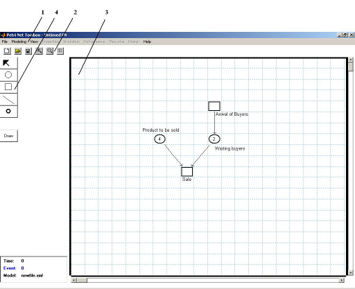
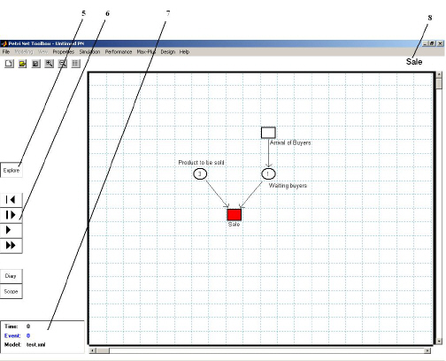
Main Features. The PN Toolbox has an easy to exploit Graphical User Interface (GUI - see fig. I.1.), whose purpose is twofold. First, it gives the user the possibility to draw PNs in a natural fashion, to store, retrieve and resize (by Zoom-In and Zoom-Out features) such drawings. Second, it permits the simulation, analysis and design of the PNs, by exploiting all the computational resources of the environment, via the global variables stored in the MATLAB’s Workspace. All the net nodes and arcs are handled as MATLAB objects so as changes in their parameters can be approached through the standard functions set and get.

When starting to build a new PN model, the user must define its type by appropriate checking in a dialogue box. The properties of the net-objects (places, transitions, arcs) depend on the selected type of model.

After drawing a PN model, the user can:

•

visualize the Incidence Matrix, which is automatically built from the net topology;

•

explore the Behavioral Properties (such as liveness, boundedness, reversibility etc.) by consulting the Coverability Tree, which is automatically built from the net topology and initial marking;

•

explore the Structural Properties (such as structural boundedness, repetitiveness, conservativeness and consistency):

•

calculate P-Invariants and T-Invariants;

•

run a Simulation experiment;

•

display current results of the simulation using the Scope and Diary facilities;

•

evaluate the global Performance Indices (such as average marking of places, average firing delay of transitions, etc.);

•

perform a Max-Plus Analysis (restricted to event-graphs);

•

Design a configuration with suitable dynamics (via automated iterative simulations).

The PN Toolbox uses the XML format for saving a model. A short description of the file format and the specific commands is given in Appendix A of this documentation.

To ensure flexibility, the set of all default values manipulated by the PN Toolbox are accessible to the user by means of a configuration file presented in Appendix B.

(a)

(b)

Fig. I.1. The main PN Toolbox window

(a) Draw Mode , (b) Explore Mode.